The computation of the global irradiation I
g on an inclined surface,
a study of dependencies has been performed to design an appropriate data
structures that optimize the memory usage of the implementation.
The calculation of global direct solar radiation under clear sky on a given
territory depends on the sun position (its altitude h
0 and longitude
A
0), the atmospheric attenuation, represented by the Linke turbidity
factor T
LK and the characteristics of the intercepting surface (its
inclination angle
d, altitude
gN,
azimuth A
N, elevation z and its horizon.
According to the latest research conducted for ESRA project, the global
irradiance can be expressed as the sum of the direct irradiance B
ic
and diffuse irradiance D
ic [
9]:
|
= I0 ·e·( Idirect+F1
·Idiffuse ) |
|
where
and
Being T
n a diffuse transmission function that depends only on the
Linke turbidity factor T
LK and F
d the diffuse solar
altitude function that dependents only on the solar altitude h
0 [
4]. K
b is the proportion
between irradiance and extraterrestrial solar irradiance on a horizontal
surface, and it depends on h
0, the number of the month m (this will
be explained in more details below in this section) and the terrain elevation z.
While, the diffuse radiation I
diffuse includes three components:
Radiation in shadow I
i, sun elevation-dependent radiation I
ii
and sun position-dependent radiation I
iii, defined as below:
|
|
|
|
|
|
|
Iiii= |
ì
ï
í
ï
î
|
|
|
|
|
Kb· sin(gN) ·cos(ALN)
/ ( 0.1-0.008 h0 )
|
|
|
|
|
|
|
|
|
where
|
|
|
F(gN)=r(gN)
·(sin(gN)-gN ·cos(gN)
- p·sin2(gN/2))·N
|
|
|
|
|
N =
|
ì
ï
í
ï
î
|
|
0.00263-0.712 ·Kb -0.6883
·K2b
|
|
|
|
|
|
|
|
|
|
|
|
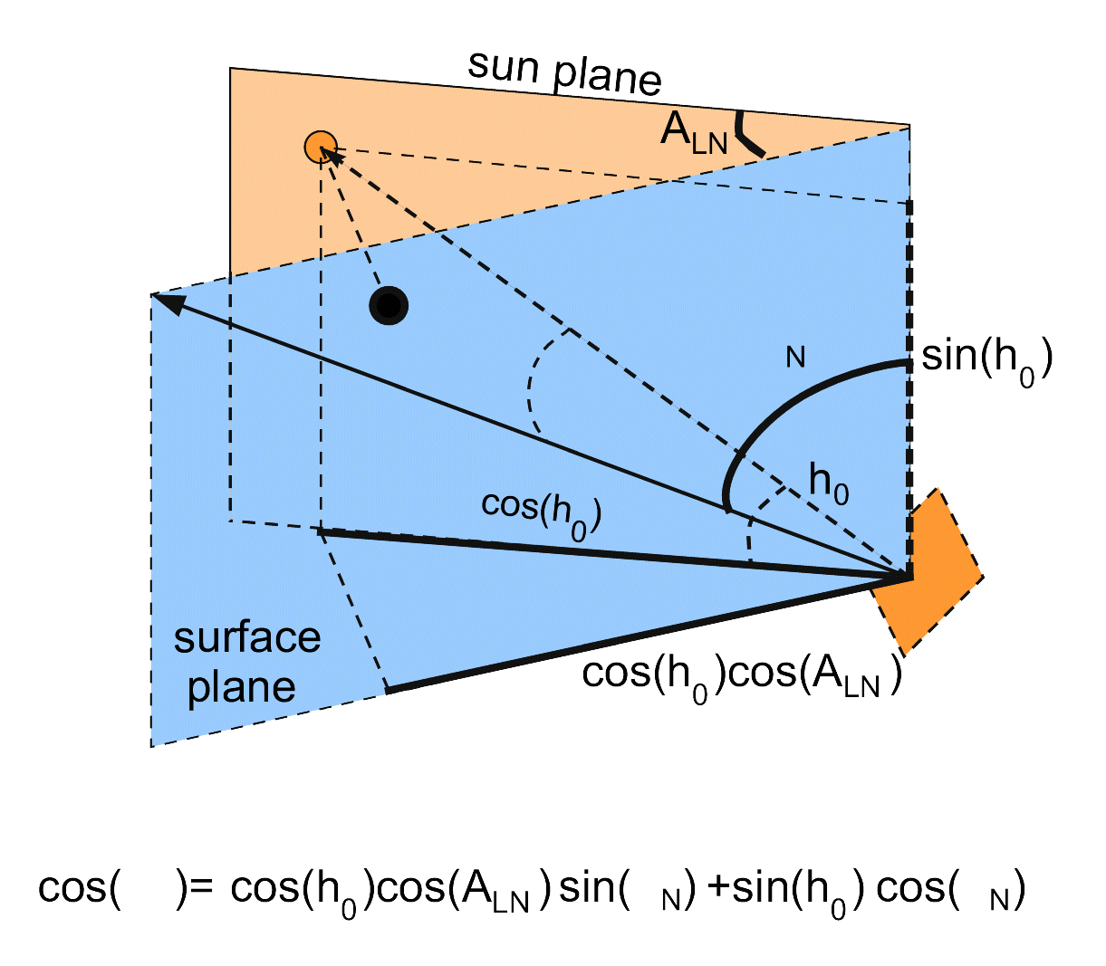
where A
LN=A
0-A
N.
As shown, the formulation of F(
gN) varies
if the sun is above or below the horizon. Moreover, the component I
iii
is different during the sunset and sunrise.
By introducing the following boolean coefficients:
lshad
(1 if the sun is below the horizon, 0 otherwise) and
ltwi
(1 if the sun elevation is lower than 5.7º, 0 otherwise) ,I
g can be
formulated as follows:
|
Ig=I0 ·e·[ Id ·cos(d) ·{1+\cfracF1 ·(1-ltwi)sin(h0) } +F1·{ Ii+Iii
+Itiii } ]
|
|
(2) |
where
I
direct=(1
-lshad)
·K
b,I
i=
lshad ·F(
gN,
lshad),I
ii
= (1
-lshad) ·(1
-K
b) ·F(
gN,
lshad),I
tiii = (1
-lshad) ·
ltwi·K
b ·\cfrac sin(
gN) ·cos(A
LN)0.1
-0.008 h
0
At a given instant, the radiation on the underlined surface can be represented
as follows:
|
Ig = I0 · |
end
å
t=ini
|
{ Id ·cos(d) ·(1+ \cfracF1 ·(1-ltwi)sin(h0))+F1
·Ii +F1 ·Iii +F1 ·Itiii
} ·e·Dt
|
|
(4) |
In most existing models, the insolation is computed using the above procedure
for every terrain cell, which means that the computational cost is proportional
to the time length and precision. In this work, an alternative integration
method is proposed, which in addition to reduce substantially the computational
cost it is almost independent on the irradiated time length and precision.
Since 0
£ h
0 £
90
° and 0
£ A
0
£ 360
°, our
first simplification consists in constructing a celestial map of hemispherical
shape that covers the considered surface. We discretize this map into N
s=90
×360 windows along the angular coordinates, altitude and azimuth. It can be
easily seen that expression
4 can be evaluated by grouping
its terms in each window. In each group, we can accumulate the global energy
received by the surface each time the sun is placed in that position in the sky.
For a discretization window of 1 ×1 degree step, I
g can be expressed
as:
I
g = I
0 ·
åA0=0360º
åh0=090º [
åk=1k=ni,j { ... }
e·
Dt ]
where n
i,j is the number of times the sun has passed from the window
{i,j}. Although the radiation must be computed for every ground cell using the
above formula, in many cases we can reuse calculations.
In a first step, some approximations are going to be assumed. The first one is
to consider that the atmosphere turbidity only depends slightly on time. That
is, we can suppose that T
LK only changes every month.
I
g = I
0 ·
åA0=0360º
{T
1+T
2+T
3+T
4+T
5 } ·
e·
Dt
T
1=cos(
gN) ·
åh0=hor90º
åm=112 n
i,j ·sin(h
0)
·K
b·(1+\cfracF
1 ·(1
-ltwi)sin(h
0))
T
2=cos(A
LN) ·sin(
gN)
·
åh0=hor90º
åm=112 n
i,j ·cos(h
0)
·K
b·(1+\cfracF
1 ·(1
-ltwi)sin(h
0))
T
3 = F(
gN,1) ·
åh0=0hor F
d(h
0)
åm=112 n
i,j ·T
n(m)
T
4=
åh0=hor90º
·
åm=112 n
i,j ·F(
gN,0) ·F
1 ·(1
-
k
b)
T
5=sin(
gN) ·cos(A
LN)
·
åh0=hor5.7
åm=112 n
i,j ·\cfracF
1
·K
b0.1
-0.008 ·h
0
where
ltwi=
ltwi(h
0),
F
1=F
1(h
0,m,z), K
b=K
b(h
0,m,z),
n
i,j=n
i,j(h
0,A
0) and a
LN
is the difference between A
0 and A
N. The calculation of
the three terms, T
1, T
2, T
3, T
4 and
T
5 is realized in three phases. In the first phase, while the sun
trajectory is calculated, one can know for each specific time interval, the
value of n
i,j in each window. We obtain the following matrices:
Arr
1(z,A
0,h
0)=
åm=112
n
i,j ·sin(h
0) ·K
b·(1+\cfracF
1 ·(1
-ltwi)sin(h
0))
)
Arr
2(z,A
0,h
0)=
åm=112
n
i,j ·cos(h
0) ·K
b·(1+\cfracF
1 ·(1
-ltwi)sin(h
0))
)
Arr
3(A
0,h
0)=F
d(h
0) ·
åm=112 n
i,j ·T
n(m)
Arr
4(z,A
0,h
0,m)=n
i,j ·F
1·(1
- k
b)
Arr
5(z,A
0,h
0)=
åm=112
n
i,j ·\cfracF
1 ·K
b0.1
-0.008
·h
0
In this phase that is independent on the terrain, these data structures are
calculated for all possible z. If the terrain is known, the calculation can be
restricted to the altitude limits of the territory z
min and z
max.
The computation in this phase depends on the period of insolation. However, even
for very small steps, of 1 minute for instance, during one year, represents a
very small fraction of the total calculation time, from 1 to 2 seconds. This
makes the total cost of our algorithm independent on the period of insolation.
When the terrain is known, we proceed to compute the following structures in the
second phase:
Arr
1b(z,A
0,hor)=
åh0=hor90º
Arr
1(z,A
0,h
0)
Arr
2b(z,A
0,hor)=
åh0=hor90º
Arr
2(z,A
0,h
0)
Arr
3b(A
0,hor) = F
d(h
0)·
åh0=0hor Arr
3(A
0,h
0)
Arr
4b(z,
gN,A
0,hor)=
åh0=hor90º F(
gN,0) ·
åm=112
Arr
4(z,A
0,h
0,m),
"gN
Arr
5b(z,A
0,hor)=
åh0=hor5.7
Arr
5(z,A
0,h
0)
where hor is the horizon; more details about its calculation is presented in
details in subsection.
As these arrays are computed for all possible values of hor, A
0,
gN and z, the execution time of this phase
only depends on the precision and the height limits z
min and z
max
of the terrain. The z-dimension of the arrays depends on the height limits and
on the height-step, 100 or 200 meters. Note that these arrays has been carefully
dimensioned. Their sizes are small enough to be held in most main memories. The
sizes are almost independent of the terrain dimensions and they ensure a fast
computation of the global insolation. Some arrays may include an additional
dimension to reduce computation, but its sizes will grow and they could be
untractable in many systems. Otherwise, the last dimension (hor) can be easily
eliminated, and both memory and computational speed will be reduced in a factor
equal to the discretization step in h
0. For a precision of one degree
in arcs, and 5 height-steps equal to 200 meter, typical execution times takes
about 8 seconds, and the memory usage is about 60MB. When the precision in the
azimuth in degree is reduced to 2 or 4, both memory usage and runtime are
reduced in the same factor and the result change slightly, we get a typical
deviation of about 2 to 7 J/m
2 in one year. Therefore, we choose a
precision of azimuth equal to 2.
Finally, the proposed insolation computation implementation can be summarized as
follows:
For x=0, gridx
-1
For y=0, gridy
-1 /* Notice that
AN and
gN are known at
this stage */
For A
0=0, 360
°
val1+=arr
1b
val2+=arr
2b ·cos(aln)
val3+=arr
3b
val4+=arr
4b
val5+=arr
5b ·cos(aln)
End For
Rg=val1 ·sin(
gN)+val2 ·cos(
gN)+val3 ·F(
gN)+val4+val5
·sin(
gN)
End For
End For
The raster maps of monthly averages values of the Linke turbidity factor T
LK
have been constructed using SoDa global database
(http://www.soda-is.com/eng/index.html). The global irradiation for real-sky
conditions was calculated using the clear-sky radiation G
hc and the
clear-sky index k
c.
For the European subcontinent, the climatologic database for 566 meteorological
stations was available (source ESRA), comprising geographical position and
monthly means of global G
hs, direct B
hs and diffuse D
hs
irradiation on a horizontal surface. The clear-sky index k
c in this
case expresses the ratio between monthly averages of global irradiation for
real-sky and computed clear-sky conditions. For each meteorological station, the
k
c was calculated using this equation: